来源:21世纪经济报道前几天一下班,就接到快毕业在找工作的表妹的电话哭诉:“为什么简历上同样写的都是“精通Excel”,面试的公司却选择了她的同学!”细细询问之下,原来面试官针对简历上的这一点,问了他们同样的问题:你们的Excel能精通到什么程度?

表妹回答说“做表格跟基本的统计吧”;她的同学表示“会Vlookup函数与透视表的程度,做可视化的图表也没有问题”,并且哗啦啦地掏出了自己做过的报告给面试官。
没有对比就没有伤害,表妹这下子可是对“精通Excel”有了深刻的认识要知道,是否真的掌握了Excel,并不是简单地在简历上写上“精通”二字就可以了01Excel堪称求职的必备技能之一,早已成为学习与工作常用的工具。
作为一个必备工具,它强大的地方就是在于,一旦熟练掌握,你所收获的将会远远超过当时学习所付出的时间与成本“你的数据,还要多久,才能整理好?”这大概是从前的我每天听到最多,也最害怕听到的一句话了其他同事早就把整理好的数据发到群里了,而我还在低头拼命地算,领导也一直在死命地催。
这感觉就像回到了高考,马上就要收卷了,可卷子还有好多好多空白,只能狂写……

大学刚毕业,作为一个运营小白,统计数据是每天的工作基本操作可别人十几分钟就能轻松搞定的事情,我常常需要几个小时才能勉强完成刚开始,我以为自己只是不熟练,多做几次就好了可闷头苦练了一个周,我还是全组最慢的那个,每天被催到怀疑人生。
“就差你的了,复制粘贴,再统计一下就好啦,怎么搞得这么慢!”渐渐地,我察觉到,领导开始质疑我的工作能力了面对这样的状况,我急忙向同事请教他们快速整理数据的秘诀没有对比,就没有伤害同事直接用Excel的公式进行计算,敲几下键盘,点几下鼠标,就轻松地把整个表格顺利完成了。

而我是用计算器一个空格一个空格地算,然后再把结果填表的!
回想起读书时,舍友选修了一门Excel课程,我还一脸不可置信地问:“Excel就填个数据,做个表格,还需要特意去学?”现在想想,当初还是太单纯了,只接触了1%的内容,就以为掌握了100%的Excel了解了我的统计方法,老大拍了拍我的肩,语重心长地说:“Excel是职场必备技能啊,你还是要多学学的……”
做行政,你要学会做考勤表;做财务,你要学会做财会报表;做销售,你要学会做销售业绩表;做运营,你要数据分析、工作汇报;……职场竞争越来越激烈,熟练掌握Excel,不能保证升职加薪,走上人生巅峰,但至少可以让你少做些无用功,少加点班,少被领导嫌弃。
02通过系统的钻研学习,现在回头看来,学Excel真的不难,比如,稍微花点心思,掌握几个简单的技巧,效率就可以提高几百个海拔“求和”,在日常工作中可以说是遇到得相当高频的一个操作了,像一个普通的表,要分别按行、按列求和:。
“一般操作”会是这样:一、用sum函数对行求和;二、下拉公式,算出所有行小计;三、再用sum函数对列求和;四、向左拖拉公式,算出所有列小计这个过程,熟手做下来,大概也要耗费30秒左右当然,不知道Sum函数的情况下,可能会有这样的“二般操作”:。
“二般操作”大概是这样:一、把行上的数据一个个加起来;二、下拉公式,算出所有行小计;三、把列上的数据一个个加起来;四、向左拖拉公式,算出所有列小计这个例子数据量不大,如果数据翻倍,用加法一个个加的速度,至少是前一种方法的一倍以上,也就是至少要1分钟,而前一种方法与数据量关系不大,速度影响也不大。
但真正的Excel其实存在一种操作:“自动求和”。
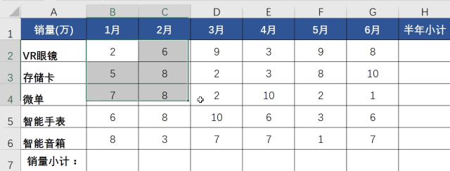
“神般操作”会是这样:一、选中要求和的空白区域;二、同时按下“ALT”和”=“键 ,即ALT+=。1秒搞定,完美!神一样的完美!来看下这3种方法的对比:

如果你是“一般”用户,那“神般”操作能帮你节省29秒,效率提高30倍如果你是“二般”用户,那能帮你节省59秒,效率提高60倍这还只是最简单的一个表,现实工作中的表比这数据量大上5~5000倍都正常,那能提高的效率就是300~300,000倍。
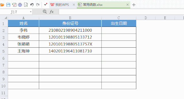
你所要学的不过是,按个快捷键“ALT+=”,就这么简单按个按钮,就提高30万倍的效率!到哪儿找,投入产生比高到如此,令!人!发!指!的事情啊!又比如:行政在统计员工信息时,如何自动获取出生日期?直接用“MID”指令截取字符串就可以方便获取,根本不需要一个一个的逐个去输入!。
掌握Excel,到底有多好?——工作上,学好Excel就等同于有了一把所向披靡的武器,应付老板各种个性化需求得心应手,还怕升职加薪轮不到你吗?简历上,增光添彩,别人的一句“精通Excel”,你却可以写上“熟练掌握VLOOKUP、IF、FIND等函数,会用数据透视表进行统计分析......”
团队合作上,熟练掌握职场必备技能Excel,自己的工作不求人还能帮助同事,职场小红人称号GET;面对一堆繁琐的数字,再也不用熬夜加班,私人时间自然就多了!03每个被Excel折磨过的人,都知道它的重要性。
可是要面对一堆繁冗复杂的函数,就算买了一堆厚厚的技术指导书,也不知道从何学起?记不住Excel的操作方法,数据一环套一环,用错方法算出来的结果天差地别,错漏百出!精通Excel其实并不难,现在行动起来并不晚!彻底告别被数据搞晕的日子,提高工作效率,实现加薪不加班!
识库君就有这样的一位朋友,对Excel了如指掌,操作的熟练程度可以说是到了炉火纯青的境界这次,识库君邀请到了微软MOS认证专家陈世杰老师,为大家开设一门《零基础Excel实战速成班,76节课从入门到精通让你效率飞起来》视频课程,立足真实场景的复杂数据,教授Excel处理方法,提升你的竞争力。

-陈世杰-微软MOS认证专家Excel工作室创始人国家注册会计师、税务师上市公司高级财务经理微软MOS认证专家:Microsoft Office Specialist(MOS),微软为全球所认可的Office软件国际性专业认证,全球有168个国家地区认可。
而陈世杰老师,是被微软MOS认证的专家
国家注册会计师、税务师、上市公司高级财务经理:陈世杰老师的经历,让他拥有丰富的实战经验,更熟悉Excel在日常学习、工作中的实际应用场景,保证你学到的Excel技能都可以落地实用。

Excel工作室创始人:陈世杰老师开设线上线下课程上百次,累计培训学员近万人。这让他十分了解学员学习Excel的痛点、重点、难点在哪儿,了解学员的实际需求,对症下药,保证学员获得最佳的学习效果。

零基础Excel实战速成,76节精致视频课6大模块,100个知识点涵盖90%职场使用场景视频讲解+配套习题+实用模板5-10分钟掌握一个核心技巧从最基本的数据录入到数据可视化提升数据处理能力,培养数据化思维
提升百倍工作效率,这一门课就够了!赠送价值199元实用Excel模板1000例!识库限时特惠价99元原价299元76节课+100个知识点+1000例模板,仅需99元(99元/76节≈1.3元=一个棒棒糖的价格)
搞定Excel升职加薪,马上点击订阅课程▼

课程到底有多超值?往下看!76节精致视频课程大纲

课程特色
零基础Excel实战速成,76节精致视频课6大模块,100个知识点涵盖90%职场使用场景视频讲解+配套习题+实用模板5-10分钟掌握一个核心技巧从最基本的数据录入到数据可视化提升数据处理能力,培养数据化思维
提升百倍工作效率,这一门课就够了!赠送价值199元实用Excel模板1000例!识库限时特惠价99元原价299元76节课+100个知识点+1000例模板,仅需99元(99元/76节≈1.3元=一个棒棒糖的价格)
搞定Excel升职加薪,马上点击订阅课程▼
学演讲、绘画或许尚需天赋学Excel,盘它就够了!■ 本课程为“视频”课程,共76期正课,由主讲人陈世杰老师亲述,全部课程已更新完毕。举报/反馈
亲爱的读者们,感谢您花时间阅读本文。如果您对本文有任何疑问或建议,请随时联系我。我非常乐意与您交流。


发表评论:
◎欢迎参与讨论,请在这里发表您的看法、交流您的观点。